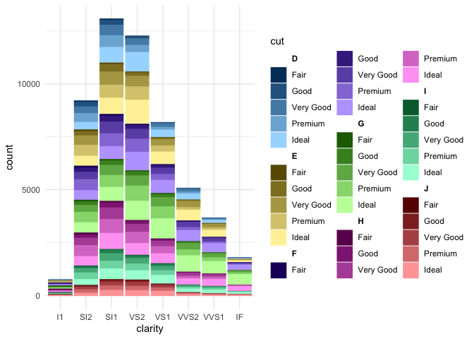
ggnested
ggnested is a wrapper function around ggplot2 that enables users to
display data with a two-level nested or clustered structure. It uses
colours or fills to label the main group or cluster, and a gradient of
shades and tints of each colour to label subgroups within each main
group. It is particularly useful for data with a hierarchy, such as
taxonomic annotations or geographic locations.
This is one of the core functions of the fantaxtic package, which
visualizes taxonomic ranks of amplicon sequencing / microbiome data as
stored in phyloseq objects. However, as it has utility beyond
displaying taxonomic annotations, it has been implemented as a separate
package.
Keywords: R, ggplot2, nested data, clustered data, multiple levels, shades, tints, gradient
Installation
if(!"devtools" %in% installed.packages()){
  install.packages("devtools")
}
devtools::install_github("gmteunisse/ggnested")
Usage
Basic
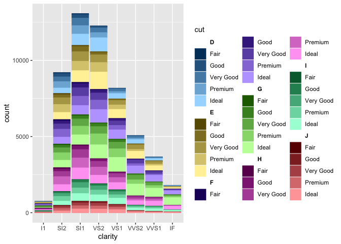
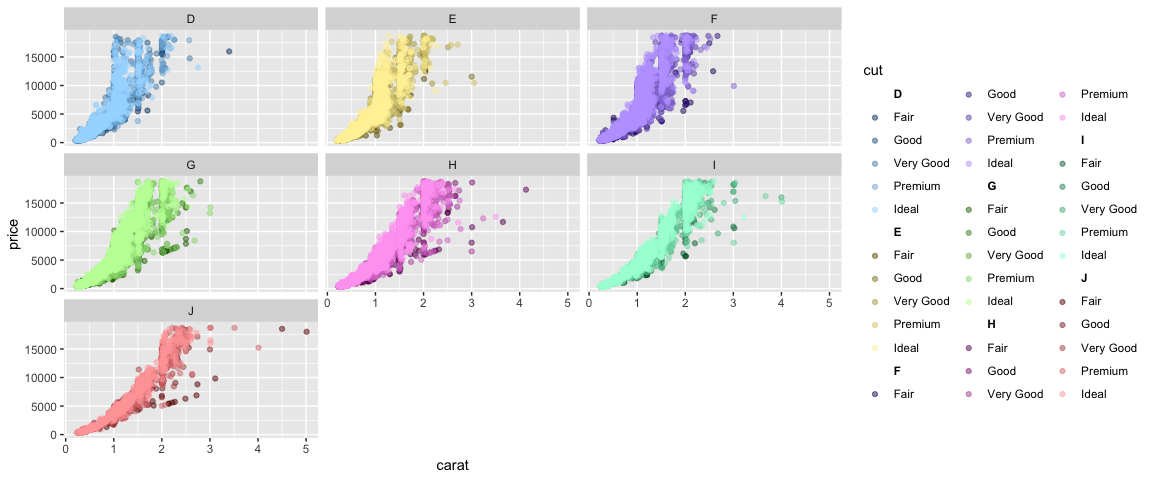
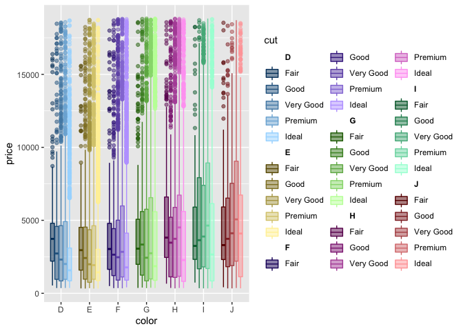
ggnested can be used exactly like the regular ggplot function, but
with some extra arguments. Instead of specifying a color or a fill, a
main_group and a sub_group need to be specified in the aesthetic
mapping through aes(...). The ggplot object can then be used to create
any regular ggplot plot, such as barplots, scatterplots or boxplots, as
well as any other layers such as faceting.
library(ggnested)
data(diamonds)
ggnested(diamonds,
         aes(clarity,
             main_group = color,
             sub_group = cut)) +
  geom_bar()
ggnested(diamonds,
         aes(x = carat,
             y = price,
             main_group = color,
             sub_group = cut)) +
  geom_point(alpha = 0.5) +
  facet_wrap(~color)
ggnested(diamonds,
         aes(x = color,
             y = price,
             main_group = color,
             sub_group = cut)) +
  geom_boxplot(alpha = .5)
Options
A few options are available, most of which are related to the appearance of the plot.
Legend
A few options are available to alter the way the legend is constructed.
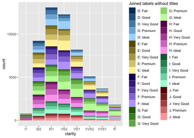
- The
legend_labelingoption alters the labels that are used in the legend. For example, it is possible to display both themain_grouplabel and thesub_grouplabel, or just themain_grouplabel. - The
join_stroption is used iflegend_labeling = "join",and specifies a string to join the two labels. - The
legend_titleoption alters the legend title. - The
main_keysdetermines whethermain_grouplabels are displayed as keys within the legend.
Bringing it all together:
ggnested(diamonds,
         aes(clarity,
             main_group = color,
             sub_group = cut),
         legend_labeling = "join",
         join_str = ": ",
         legend_title = "Joined labels without titles",
         main_keys = FALSE) +
  geom_bar()
Colour palette
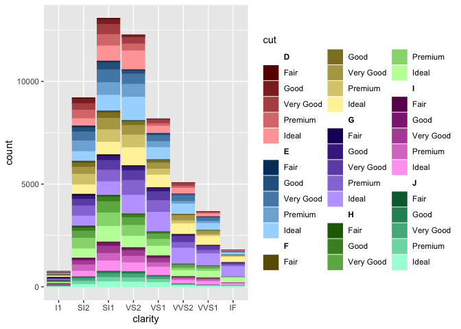
ggnested creates its own colour palettes. Like ggplot2, it samples
maximally separated colours, but unlike ggplot2, it shuffles the palette
so that dissimlar colours are placed next to one another. This is to
avoid confusion in colours and shades between different groups. Also
unlike ggplot2, the user can define a base colour
(e.g. base_clr = #008CF0) that serves as the first colour of the
palette, based on which all other colours are sampled. Finally, A custom
palette of colours for the main_group can be provided
(main_palette = c()), which will then be used to generate gradients
for the subgroups.
ggnested(diamonds,
         aes(clarity,
             main_group = color,
             sub_group = cut),
         base_clr = "red") +
  geom_bar()
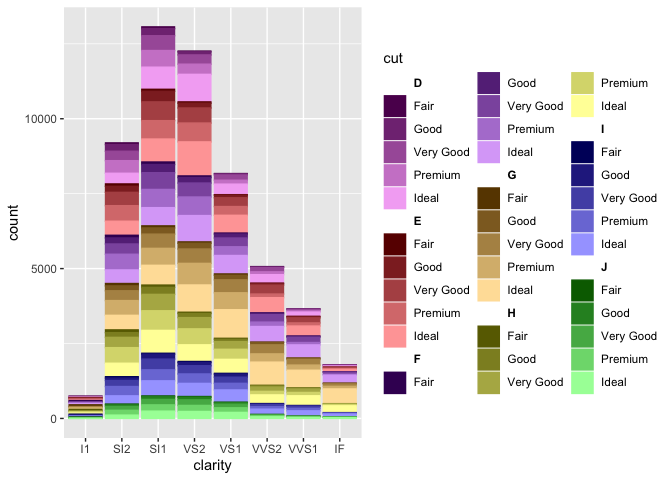
Note that if a custom palette is named, the colours will be associated
with the appropriate main_group level.
pal <- c("red", "blue", "green", "yellow", "purple", "orange", "violet")
names(pal) <- unique(diamonds$color)
p <- ggnested(diamonds,
         aes(clarity,
             main_group = color,
             sub_group = cut),
         main_palette = pal) +
  geom_bar()
p
Gradients
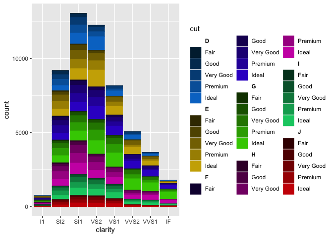
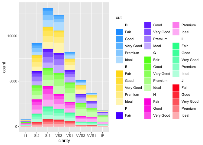
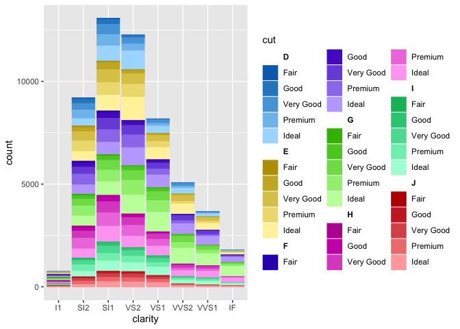
For each colour, a gradient between a dark shade and a lighter tint of
the required number of colours is generated. By default, ggnested will
generate both shades and tints for each colour. However, it is possible
to limit the gradient generation to only shades or tints. Furthermore,
it is possible to set the darkness and lightness limits of the scale.
ggnested(diamonds,
         aes(clarity,
             main_group = color,
             sub_group = cut),
         gradient_type = "shades",
         min_l = 0.05) +
  geom_bar()
ggnested(diamonds,
         aes(clarity,
             main_group = color,
             sub_group = cut),
         gradient_type = "tints",
         max_l = 0.95) +
  geom_bar()
ggnested(diamonds,
         aes(clarity,
             main_group = color,
             sub_group = cut),
         gradient_type = "both",
         min_l = 0.25,
         max_l = 0.95) +
  geom_bar()
Fancy gradients
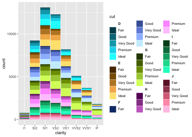
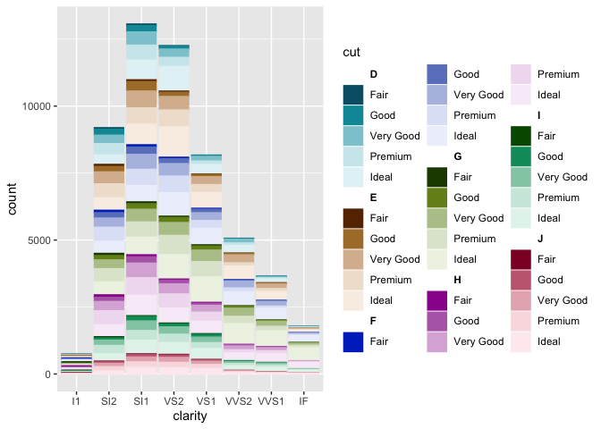
As you can tell by the plots above, the shades and tints approach can
sometimes look a bit flat. A fourth option, fancy, is therefore
available. In this mode, it is recommended to change the default min_l
to a higher number. Furthermore, some additional parameters are
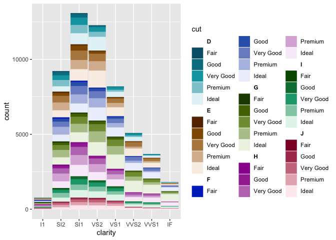
available, namely min_c, max_c and power. min_c and max_c
alter the minimum and maximum chroma of the gradient, which determines
the saturation. power determines whether the gradient is linear (1),
quadratic (2) or more.
ggnested(diamonds,
         aes(clarity,
             main_group = color,
             sub_group = cut),
         gradient_type = "fancy",
         min_l = 0.25,
         max_l = 0.95) +
  geom_bar()
ggnested(diamonds,
         aes(clarity,
             main_group = color,
             sub_group = cut),
         gradient_type = "fancy",
         min_l = 0.25,
         max_l = 0.95,
         min_c = 100,
         max_c = 10
         ) +
  geom_bar()
ggnested(diamonds,
         aes(clarity,
             main_group = color,
             sub_group = cut),
         gradient_type = "fancy",
         min_l = 0.25,
         max_l = 0.95,
         min_c = 100,
         max_c = 10,
         power=2
         ) +
  geom_bar()
Palette generation
It’s also possible to create your own nested palette for other purposes:
nested_palette(diamonds,
               group = "color",
               subgroup = "cut")
#> # A tibble: 35 × 5
#>    color cut       group_colour subgroup_colour group_subgroup
#>    <ord> <ord>     <chr>        <chr>           <chr>
#>  1 D     Fair      #008CF0      #003D69         D_Fair
#>  2 D     Good      #008CF0      #29648E         D_Good
#>  3 D     Very Good #008CF0      #538BB3         D_Very Good
#>  4 D     Premium   #008CF0      #7CB2D9         D_Premium
#>  5 D     Ideal     #008CF0      #A6DAFF         D_Ideal
#>  6 E     Fair      #F0CB00      #695800         E_Fair
#>  7 E     Good      #F0CB00      #8E7E29         E_Good
#>  8 E     Very Good #F0CB00      #B3A453         E_Very Good
#>  9 E     Premium   #F0CB00      #D9CA7C         E_Premium
#> 10 E     Ideal     #F0CB00      #FFF1A6         E_Ideal
#> # … with 25 more rows
Alternatively, the colour palette can be extracted from the ggplot2
object using extract_palette.
extract_palette(p)
#> # A tibble: 35 × 3
#>    group_subgroup group_colour subgroup_colour
#>    <ord>          <chr>        <chr>
#>  1 D - Fair       violet       #5C0D5C
#>  2 D - Good       violet       #823582
#>  3 D - Very Good  violet       #A85EA8
#>  4 D - Premium    violet       #CE87CE
#>  5 D - Ideal      violet       #F4B0F4
#>  6 E - Fair       red          #690000
#>  7 E - Good       red          #8E2929
#>  8 E - Very Good  red          #B35353
#>  9 E - Premium    red          #D97C7C
#> 10 E - Ideal      red          #FFA6A6
#> # … with 25 more rows
Affected aesthetics
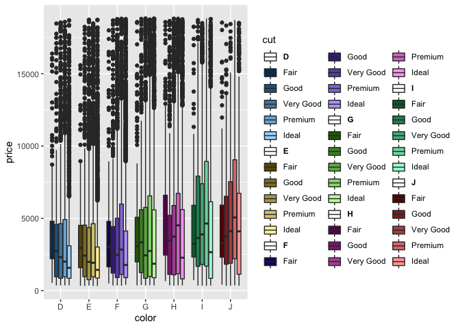
By default, both the color and fill aesthetics of the plot are
altered by ggnested. However, it is possible to specify which
aesthetics should be altered using nested_aes = c("fill", "colour").
Note that it leads to issues with the legends of geoms that
automatically create both colour and fill aethetics, as shown with
the boxplots below - the main_group titles now also show a box
outline! This can of course be resolved by setting main_keys = FALSE
as shown above.
ggnested(diamonds,
         aes(x = color,
             y = price,
             main_group = color,
             sub_group = cut),
         nested_aes = "fill") +
  geom_boxplot()
Themes
To ensure that a ggnested plot does not alter when the theme is
altered, it is recommended to alter the theme using the theme_nested
function. This function is simply a wrapper around any ggplot theme_*
function.
ggnested(diamonds,
         aes(clarity,
             main_group = color,
             sub_group = cut)) +
  geom_bar() +
  theme_nested(theme_minimal)
